I took some nerve to start the Kaggle but am really glad I did
get to start after multiple false starts.
By following this you’ll be able to score atleast top 5000th position on the leaders board.
Let’s import some libraries to get started!
import numpy as np
import pandas as pd
import matplotlib.pyplot as plt
import seaborn as sns

%matplotlib inline
sns.set_style('whitegrid')
The Data
We will be working with the Titanic Data Set from Kaggle downloaded as train.csv file
train = pd.read_csv('train.csv')
test_df = pd.read_csv('test.csv')

train.head(2)
| PassengerId | Survived | Pclass | Name | Sex | Age | SibSp | Parch | Ticket | Fare | Cabin | Embarked | |
|---|---|---|---|---|---|---|---|---|---|---|---|---|
| 0 | 1 | 0 | 3 | Braund, Mr. Owen Harris | male | 22.0 | 1 | 0 | A/5 21171 | 7.2500 | NaN | S |
| 1 | 2 | 1 | 1 | Cumings, Mrs. John Bradley (Florence Briggs Th... | female | 38.0 | 1 | 0 | PC 17599 | 71.2833 | C85 | C |
Exploratory Data Analysis
Some exploratory data analysis!
We’ll start by checking out missing data!
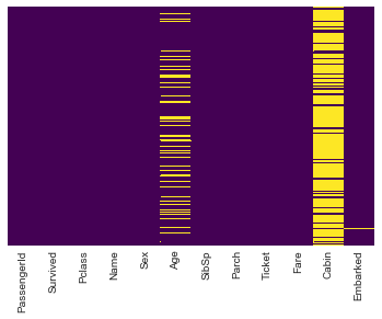
Missing Data
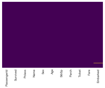
We can use seaborn to create a simple heatmap to see where we are missing data!
sns.heatmap(train.isnull(),yticklabels=False,cbar=False,cmap='viridis')

# An assessment of data available, Age and Cabin have missing values while the rest
# are relatively OK.
Visualizing some more of the data
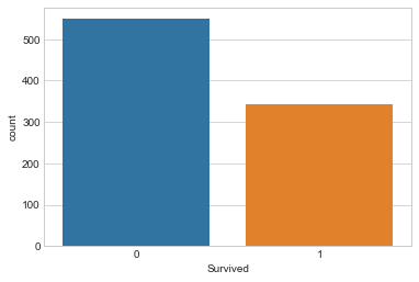
analysis by column. By Survival
sns.countplot(x='Survived',data=train)
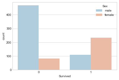
Survival by Gender
sns.countplot(x='Survived',hue='Sex',data=train,palette='RdBu_r')
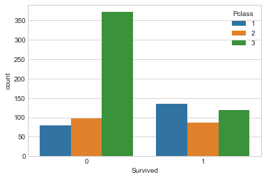
Survival by Passenger Class
sns.countplot(x='Survived',hue='Pclass',data=train)
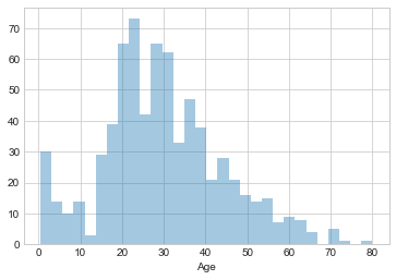
Distribution of Passengers on board by Age
sns.distplot(train['Age'].dropna(),kde=False,bins=30)
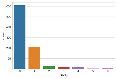
Passengers onboard with sibling(s) / spouse
sns.countplot(x='SibSp',data=train)
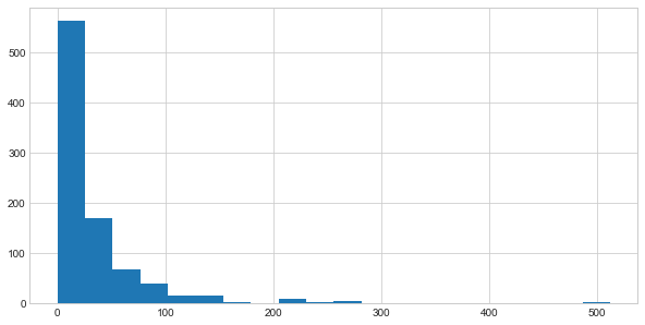
Passengers by amount of fare paid
train['Fare'].hist(bins=20,figsize=(10,5))
Data Cleaning
Imputation.
- Filling out missing values by approximation
- Fill in the mean age to the age column
Start of by checking the average age by passenger class.
plt.figure(figsize=(10,7))
sns.boxplot(x='Pclass',y='Age',data=train)
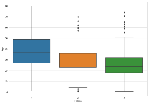
Wealthier passengers in the higher classes tend to be older,
We’ll use these average age values to impute missing data based on Pclass for Age.
def impute_age(cols):
    Age = cols[0]
    Pclass = cols[1]

    if pd.isnull(Age):
        if Pclass == 1:
            return 37
        elif Pclass == 2:
            return 29
        else:
            return 24

    else:
        return Age
Apply impute_age function
train['Age'] = train[['Age','Pclass']].apply(impute_age,axis=1)
And by checking for missing values on our data, we have;
sns.heatmap(train.isnull(),yticklabels=False,cbar=False,cmap='viridis')
We can Drop the Cabin column as it possesses a huge percentage of missing values and filling
in may not be appropriatte.
Also we will drop the few instances on the Embarked column
# train.drop('Cabin',axis=1,inplace=True)
Check that the dataset has been well preprocessed.
train.info()
<class 'pandas.core.frame.DataFrame'>
RangeIndex: 891 entries, 0 to 890
Data columns (total 11 columns):
PassengerId    891 non-null int64
Survived       891 non-null int64
Pclass         891 non-null int64
Name           891 non-null object
Sex            891 non-null object
Age            891 non-null float64
SibSp          891 non-null int64
Parch          891 non-null int64
Ticket         891 non-null object
Fare           891 non-null float64
Embarked       889 non-null object
dtypes: float64(2), int64(5), object(4)
memory usage: 76.6+ KB
Convert Categorical Features
We need to convert categorical features to dummy variables using pandas,
Otherwise the learning algorithm won’t be able to directly take in those features as inputs.
| For the sex column, caterorize if passenger is male or not(1 | 0 ) |
On embarkment point it will be Q, S 0r C.
sex = pd.get_dummies(train['Sex'],drop_first=True)

embark = pd.get_dummies(train['Embarked'],drop_first=True)
Concatenate the generated categorical columns to the dataset
train = pd.concat([train, sex,embark],axis=1)
train.head(2)
| PassengerId | Survived | Pclass | Name | Sex | Age | SibSp | Parch | Ticket | Fare | Embarked | male | Q | S | |
|---|---|---|---|---|---|---|---|---|---|---|---|---|---|---|
| 0 | 1 | 0 | 3 | Braund, Mr. Owen Harris | male | 22.0 | 1 | 0 | A/5 21171 | 7.2500 | S | 1 | 0 | 1 |
| 1 | 2 | 1 | 1 | Cumings, Mrs. John Bradley (Florence Briggs Th... | female | 38.0 | 1 | 0 | PC 17599 | 71.2833 | C | 0 | 0 | 0 |
Select Columns that we will use for the model
train.drop(['Name','Sex','Embarked','Ticket'],axis=1,inplace=True)
# train.drop('PassengerId',axis=1,inplace=True)
train.head(2)
| Survived | Pclass | Age | SibSp | Parch | Fare | male | Q | S | |
|---|---|---|---|---|---|---|---|---|---|
| 0 | 0 | 3 | 22.0 | 1 | 0 | 7.2500 | 1 | 0 | 1 |
| 1 | 1 | 1 | 38.0 | 1 | 0 | 71.2833 | 0 | 0 | 0 |
Prep the test Set
test_df.info()
<class 'pandas.core.frame.DataFrame'>
RangeIndex: 418 entries, 0 to 417
Data columns (total 9 columns):
PassengerId    418 non-null int64
Pclass         418 non-null int64
Age            418 non-null float64
SibSp          418 non-null int64
Parch          418 non-null int64
Fare           418 non-null float64
male           418 non-null uint8
Q              418 non-null uint8
S              418 non-null uint8
dtypes: float64(2), int64(4), uint8(3)
memory usage: 20.9 KB
test_df['Fare'].fillna(test_df['Fare'].mean(), inplace=True)
test_df['Age'].fillna(test_df['Age'].mean(), inplace=True)
sex_t = pd.get_dummies(test_df['Sex'],drop_first=True)

embark_t = pd.get_dummies(test_df['Embarked'],drop_first=True)
test_df = pd.concat([test_df, sex_t,embark_t],axis=1)
test_df.drop(['Name','Sex','Embarked','Ticket','Cabin'],axis=1,inplace=True)
test_df.head(2)
| PassengerId | Pclass | Age | SibSp | Parch | Fare | male | Q | S | |
|---|---|---|---|---|---|---|---|---|---|
| 0 | 892 | 3 | 34.5 | 0 | 0 | 7.8292 | 1 | 1 | 0 |
| 1 | 893 | 3 | 47.0 | 1 | 0 | 7.0000 | 0 | 0 | 1 |
test_df.head(2)
| PassengerId | Pclass | Age | SibSp | Parch | Fare | male | Q | S | |
|---|---|---|---|---|---|---|---|---|---|
| 0 | 892 | 3 | 34.5 | 0 | 0 | 7.8292 | 1 | 1 | 0 |
| 1 | 893 | 3 | 47.0 | 1 | 0 | 7.0000 | 0 | 0 | 1 |
And the data is ready for our model!
Building a Logistic Regression model
Start by splitting data into a training set and test set
Train Test Split
X = These are the features we will use to predict

y = Value we are predicting ie Did the passenger survive
X = train.drop('Survived',axis=1)
y = train['Survived']
Prep the test dataset
from sklearn.model_selection import train_test_split
X_train = train.drop('Survived',axis=1)
y_train = train['Survived']
X_train.info()
<class 'pandas.core.frame.DataFrame'>
RangeIndex: 891 entries, 0 to 890
Data columns (total 8 columns):
Pclass    891 non-null int64
Age       891 non-null float64
SibSp     891 non-null int64
Parch     891 non-null int64
Fare      891 non-null float64
male      891 non-null uint8
Q         891 non-null uint8
S         891 non-null uint8
dtypes: float64(2), int64(3), uint8(3)
memory usage: 37.5 KB
X_test = test_df.drop('PassengerId',axis=1)
X_test.info()
<class 'pandas.core.frame.DataFrame'>
RangeIndex: 418 entries, 0 to 417
Data columns (total 8 columns):
Pclass    418 non-null int64
Age       418 non-null float64
SibSp     418 non-null int64
Parch     418 non-null int64
Fare      418 non-null float64
male      418 non-null uint8
Q         418 non-null uint8
S         418 non-null uint8
dtypes: float64(2), int64(3), uint8(3)
memory usage: 17.6 KB
Training and Predicting
from sklearn.linear_model import LogisticRegression
Create an instance of Linear Regression model
logmodel = LogisticRegression()
Train the model
logmodel.fit(X_train,y_train)
LogisticRegression(C=1.0, class_weight=None, dual=False, fit_intercept=True,
          intercept_scaling=1, max_iter=100, multi_class='ovr', n_jobs=1,
          penalty='l2', random_state=None, solver='liblinear', tol=0.0001,
          verbose=0, warm_start=False)
Make Predictions using the model
predictions = logmodel.predict(X_test)
Generate Submission File
The Kaggle evaluation will be based upon the Predictions made in reference to ‘PassengerId` from the test.csv
Submission = pd.DataFrame({ 'PassengerId': test_df['PassengerId'],
                            'Survived': predictions })
Submission.to_csv("4bic_titanic_submission.csv", index=False)
I got an accuracy of 0.706,, find ways to improve